Interpreting Odds Ratios for Continuous Variables in Logistic Regression
- This presentation presents a broad overview of methods for interpreting interactions in logistic regression.
- The presentation is not about Stata. It uses Stata, but you gotta use something.
- The methods shown are somewhat stat package independent. However, they can be easier or more difficult to implement depending on the stat package.
- The presentation is not a step-by-step how-to manual that shows all of the code that was used to produce the results shown.
- Each of the models used in the examples will have two research variables that are interacted and one continuous covariate (cv1) that is not part of the interaction.
Some Definitions
Odds
Showing that odds are ratios.
odds = p/(1 - p)
Log Odds
Natural log of the odds, also known as a logit.
log odds = logit = log(p/(1 - p))
Odds Ratio
Showing that odds ratios are actually ratios of ratios.
odds1 p1/(1 - p1) odds_ratio = ----- = ------------- odds2 p2/(1 - p2)
Computing Odds Ratio from Logistic Regression Coefficient
odds_ratio = exp(b)
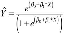
Computing Probability from Logistic Regression Coefficients
probability = exp(Xb)/(1 + exp(Xb))
Where Xb is the linear predictor.
About Logistic Regression
Logistic regression fits a maximum likelihood logit model. The model estimates conditional means in terms of logits (log odds). The logit model is a linear model in the log odds metric. Logistic regression results can be displayed as odds ratios or as probabilities. Probabilities are a nonlinear transformation of the log odds results.
In general, linear models have a number of advantages over nonlinear models and are easier to work with. For example, in linear models the slopes and/or differences in means do not change for differing values of a covariate. This is not necessarily the case for nonlinear models. The problem in logistic regression is that, even though the model is linear in log odds, many researchers feel that log odds are not a natural metric and are not easily interpreted.
Probability is a much more natural metric. However, the logit model is not linear when working in the probability metric. Thus, the predicted probabilities change as the values of a covariate change. In fact, the estimated probabilities depend on all variables in the model not just the variables in the interaction.
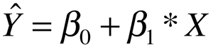
So what is a linear model? A linear model is linear in the betas (coefficients). By extension, a nonlinear model must be nonlinear in the betas. Below are three example of linear and nonlinear models.
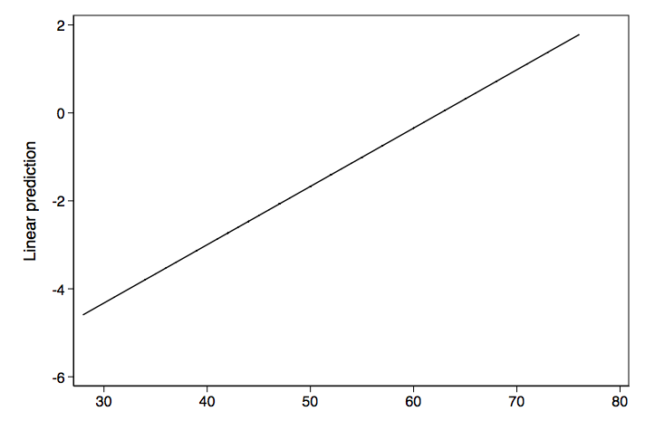
First, is an example of a linear model and its graph.
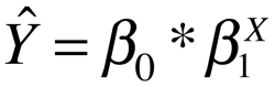
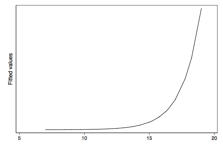
Next we have an example of a nonlinear model and its graph. In this case its an exponential growth model.
Lastly we have another nonlinear model. This one shows the nonlinear transformation of log odds to probabilities.
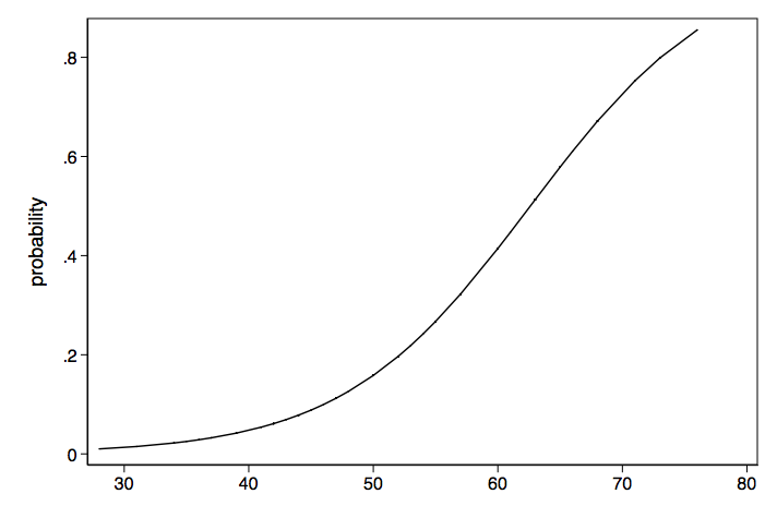
Logistic Regression Transformations
This is an attempt to show the different types of transformations that can occur with logistic regression models.
probability / / / / / / odds ratios ----- log odds ------- odds
Logistic interactions are a complex concept
Common wisdom suggests that interactions involves exploring differences in differences. If the differences are not different then there is no interaction. But in logistic regression interaction is a more complex concept. Researchers need to decide on how to conceptualize the interaction. Is the interaction to be conceptualized in terms of log odds (logits) or odds ratios or probability? This decision can make a big difference. An interaction that is significant in log odds may not be significant in terms of difference in differences for probability. Or vice versa.
Model 1: categorical by categorical interaction
Log odds metric — categorical by categorical interaction
Variables f and h are binary predictors, while cv1 is a continuous covariate. The nolog option suppresses the display of the iteration log; it is used here simply to minimize the quantity of output.
logit y01 f##h cv1, nolog Logistic regression Number of obs = 200 LR chi2(4) = 106.10 Prob > chi2 = 0.0000 Log likelihood = -78.74193 Pseudo R2 = 0.4025 ------------------------------------------------------------------------------ y01 | Coef. Std. Err. z P>|z| [95% Conf. Interval] -------------+---------------------------------------------------------------- 1.f | 2.996118 .7521524 3.98 0.000 1.521926 4.470309 1.h | 2.390911 .6608498 3.62 0.000 1.09567 3.686153 | f#h | 1 1 | -2.047755 .8807989 -2.32 0.020 -3.774089 -.3214213 | cv1 | .196476 .0328518 5.98 0.000 .1320876 .2608644 _cons | -11.86075 1.895828 -6.26 0.000 -15.5765 -8.144991 ------------------------------------------------------------------------------
The interaction term is clearly significant. We could manually compute the expected logits for each of the four cells in the model.
f h cell 0 0 b[_cons] = -11.86075 cell 0 1 b[_cons] + b[1.f] = -11.86075 + 2.390911 = -9.469835 cell 1 0 b[_cons] + b[1.h] = -11.86075 + 2.996118 = -8.864629 cell 1 1 b[_cons] + b[1.f] + b[1.h] + b[1.f#1.h] = -11.86075 + 2.390911 + 2.996118 - 2.047755 = -8.521473
We can also use a cell-means model to obtain the expected logits for each cell when cv1=0. The nocons option is used omit the constant term. Because the constant is not included in the calculations, a coefficient for the reference group is calculated.
logit y01 bn.f#bn.h cv1, nocons nolog Logistic regression Number of obs = 200 Wald chi2(5) = 50.48 Log likelihood = -78.74193 Prob > chi2 = 0.0000 ------------------------------------------------------------------------------ y01 | Coef. Std. Err. z P>|z| [95% Conf. Interval] -------------+---------------------------------------------------------------- f#h | 0 0 | -11.86075 1.895828 -6.26 0.000 -15.5765 -8.144991 0 1 | -9.469835 1.714828 -5.52 0.000 -12.83084 -6.108835 1 0 | -8.864629 1.530269 -5.79 0.000 -11.8639 -5.865356 1 1 | -8.521473 1.640705 -5.19 0.000 -11.73719 -5.30575 | cv1 | .196476 .0328518 5.98 0.000 .1320876 .2608644 ------------------------------------------------------------------------------
And here is what the expected logits look like in a 2×2 table.
| h=0 | h=1 | |
| f=0 | -11.86075 | -9.469835 |
| f=1 | -8.8646295 | -8.521473 |
We will look at the differences between h0 and h1 at each level of f (simple main effects) and also at the difference in differences.
/* difference 1 at f = 0 */ lincom 0.f#0.h - 0.f#1.h ( 1) [y01]0bn.f#0bn.h - [y01]0bn.f#1.h = 0 ------------------------------------------------------------------------------ y01 | Coef. Std. Err. z P>|z| [95% Conf. Interval] -------------+---------------------------------------------------------------- (1) | -2.390911 .6608498 -3.62 0.000 -3.686153 -1.09567 ------------------------------------------------------------------------------ /* difference 2 at f = 1 */ lincom 1.f#0.h - 1.f#1.h ( 1) [y01]1.f#0bn.h - [y01]1.f#1.h = 0 ------------------------------------------------------------------------------ y01 | Coef. Std. Err. z P>|z| [95% Conf. Interval] -------------+---------------------------------------------------------------- (1) | -.3431562 .5507722 -0.62 0.533 -1.42265 .7363375 ------------------------------------------------------------------------------
Difference 1 suggests that h0 is significantly different from h1 at f = 0, While difference 2 does not show a significant difference at f = 1. These are tests of simple main effects just like we would do in OLS (ordinary least squares) regression. We will finish up this section by looking at the difference in differences.
/* difference in differences */ lincom (0.f#0.h - 0.f#1.h)-(1.f#0.h - 1.f#1.h) ( 1) [y01]0bn.f#0bn.h - [y01]0bn.f#1.h - [y01]1.f#0bn.h + [y01]1.f#1.h = 0 ------------------------------------------------------------------------------ y01 | Coef. Std. Err. z P>|z| [95% Conf. Interval] -------------+---------------------------------------------------------------- (1) | -2.047755 .8807989 -2.32 0.020 -3.774089 -.3214213 ------------------------------------------------------------------------------
The difference in differences is, of course, just another name for the interaction. For the log odds model the differences and the difference in differences are the same regardless of the value of the covariate. This constancy across different values of the covariate is one of the properties of linear models.
Odds ratio metric — categorical by categorical interaction
Let's look at a table of logistic regression coefficients along with the exponentiated coefficients, which some people call odds ratios.
---------------------------------------------------------- source | coefficient exp(coef) type of exp(coef) --------+------------------------------------------------- f | 2.996118 20.007716 odds ratio h | 2.390911 10.92345 odds ratio f#h | -2.047755 0.1290242 ratio of odds ratios cv1 | 0.196476 1.217106 odds ratio _cons | -11.86075 7.062e-06 baseline odds ---------------------------------------------------------
Many people call all exponentiated logistic coefficients odds ratios. But as you can see from the table above, exponentiating the interaction is a ratio of ratios and the exponentiated constant is the baseline odds.
We can compute the odds ratios manually for each of the two levels of f from the values in the table above.
odds ratio h1/h0 for f=0: b[1.h] = 10.92345 odds ratio h1/h0 for f=1: b[1.h]*b[f#h] = 10.92345*.1290242 = 1.4093894
Please note that the computation of the odds ratio for f =1 involves multiplying coefficients for the odds ratio model above which implies that odds ratio models are multiplicative rather than additive.
The baseline odds when cv1 = zero is very small (7.06e-06) so for the remainder of of the computations we will estimate the odds while holding cv1 at 50. The option noatlegend suppresses the display of the legend.
margins, over(f h) at(cv1=50) expression(exp(xb())) noatlegend Predictive margins Number of obs = 200 Model VCE : OIM Expression : exp(xb()) over : f h ------------------------------------------------------------------------------ | Delta-method | Margin Std. Err. z P>|z| [95% Conf. Interval] -------------+---------------------------------------------------------------- f h | 0 0 | .1304264 .0734908 1.77 0.076 -.0136129 .2744657 0 1 | 1.424706 .515989 2.76 0.006 .4133857 2.436025 1 0 | 2.609533 1.136545 2.30 0.022 .3819457 4.837121 1 1 | 3.677847 1.311463 2.80 0.005 1.107427 6.248267 ------------------------------------------------------------------------------
The option expression(exp(xb())) insures that we are looking at results in the odds ratio metric. The baseline odds are now .1304264 which is reasonable. We will compute the odds ratio for each level of f.
odds ratio 1 at f=0: 1.424706/.1304264 = 10.923446 odds ratio 2 at f=1: 3.677847/2.609533 = 1.4093889
So when f = 0 the odds of the outcome being one are 10.92 times greater for h1 then for h0. For f = 1 the ratio of the two odds is only 1.41. These odds ratios are the same as we computed manually earlier.
We can also compute the ratio of odds ratios and show that it reproduces the estimate for the interaction.
ratio of odds ratios: (3.677847/2.609533)/(1.424706/.1304264) = .1290242
The one nice thing that we can say about working in odds ratio metric is the odds ratios remain the same regardless of where we hold the covariate constant.
Probability metric — categorical by categorical interaction
We will begin by rerunning our logistic regression model to refresh our memories on the coefficients.
logit y01 f##h cv1, nolog Logistic regression Number of obs = 200 LR chi2(4) = 106.10 Prob > chi2 = 0.0000 Log likelihood = -78.74193 Pseudo R2 = 0.4025 ------------------------------------------------------------------------------ y01 | Coef. Std. Err. z P>|z| [95% Conf. Interval] -------------+---------------------------------------------------------------- 1.f | 2.996118 .7521524 3.98 0.000 1.521926 4.470309 1.h | 2.390911 .6608498 3.62 0.000 1.09567 3.686153 | f#h | 1 1 | -2.047755 .8807989 -2.32 0.020 -3.774089 -.3214213 | cv1 | .196476 .0328518 5.98 0.000 .1320876 .2608644 _cons | -11.86075 1.895828 -6.26 0.000 -15.5765 -8.144991 ------------------------------------------------------------------------------
Let's manually compute the probability of the outcome being one for the f = 0, h = 0 cell when cv1 is held at 50.
Xb = b[_cons] + 0*b[1.f] + 0*b[1.h] + 0*b{f#h} + 50*b[cv1] = -11.86075 + 0*2.996118 + 0*2.390911 + 0*-2.047755 + 50*.196476 = -2.03695 probability = exp(Xb)/(1+exp(Xb)) = exp(-2.03695)/(1+exp(-2.03695)) = .11537767 We could repeat this for each of the other three cells but instead we we will obtain the expected probabilities for each cell while holding the covariate at 50 using the margins command.
margins f#h, at(cv1=50) Adjusted predictions Number of obs = 200 Model VCE : OIM Expression : Pr(y01), predict() at : cv1 = 50 ------------------------------------------------------------------------------ | Delta-method | Margin Std. Err. z P>|z| [95% Conf. Interval] -------------+---------------------------------------------------------------- f#h | 0 0 | .115378 .0575106 2.01 0.045 .0026592 .2280968 0 1 | .5875788 .0877652 6.69 0.000 .4155621 .7595955 1 0 | .7229559 .0872338 8.29 0.000 .5519808 .8939309 1 1 | .7862264 .0599327 13.12 0.000 .6687605 .9036924 ------------------------------------------------------------------------------
Here are the same results displayed as a table.
h=0 h=1 f=0 .115378 .5875788 f=1 .7229559 .7862264
We would like to look at the differences in h for each level of f.
h1 - h0 at f = 0: .5875788 - .115378 = .4722008 h1 - h0 at f = 1: .7862264 - .7229559 = .0632706
We can also do this with a slight variation of the margins command and get estimates of the differences in probability along with standard errors and confidence intervals.
margins f, dydx(h) at(cv1=50) post Conditional marginal effects Number of obs = 200 Model VCE : OIM Expression : Pr(y01), predict() dy/dx w.r.t. : 0.h 1.h at : cv1 = 50 ------------------------------------------------------------------------------ | Delta-method | dy/dx Std. Err. z P>|z| [95% Conf. Interval] -------------+---------------------------------------------------------------- 1.h | f | 0 | .4722008 .1035128 4.56 0.000 .2693195 .675082 1 | .0632706 .1036697 0.61 0.542 -.1399183 .2664595 ------------------------------------------------------------------------------ Note: dy/dx for factor levels is the discrete change from the base level.
These two differences are the probability analogs to the simple main effects from the log odds model. So, when the covariate is held at 50 there is a significant difference in h at f = 0 but not at f = 1.
Next, we will use lincom to compute the difference in differences when cv1 is held at 50.
lincom [1.h]0.f-[1.h]1.f ( 1) [1.h]0bn.f - [1.h]1.f = 0 ------------------------------------------------------------------------------ | Coef. Std. Err. z P>|z| [95% Conf. Interval] -------------+---------------------------------------------------------------- (1) | .4089302 .1482533 2.76 0.006 .118359 .6995014 ------------------------------------------------------------------------------
The p-value here is different form the p-value from the original logit model because in the probability metric the values of the covariate matter.
If we repeat the above process for values of cv1 from 20 to 70, we can produce a table of simple main effects and a graph of the difference in differences.
Table of Simple Main Effects for h at Two Levels of f for Various Values of cv1 | Delta-method | dy/dx Std. Err. z P>|z| [95% Conf. Interval] -------------+---------------------------------------------------------------- cv1 f | 20 0 | .0035507 .0038256 0.93 0.353 -.0039472 .0110487 20 1 | .002893 .0057719 0.50 0.616 -.0084197 .0142058 30 0 | .0246805 .0188412 1.31 0.190 -.0122475 .0616086 30 1 | .0186252 .0331697 0.56 0.574 -.0463863 .0836367 40 0 | .1485222 .0656193 2.26 0.024 .0199107 .2771337 40 1 | .0723494 .1167547 0.62 0.535 -.1564856 .3011843 50 0 | .4722008 .1035128 4.56 0.000 .2693195 .675082 50 1 | .0632706 .1036697 0.61 0.542 -.1399183 .2664595 60 0 | .4284548 .137549 3.11 0.002 .1588636 .6980459 60 1 | .0142654 .0255894 0.56 0.577 -.0358888 .0644197 70 0 | .1173445 .076704 1.53 0.126 -.0329926 .2676816 70 1 | .0021597 .0042758 0.51 0.613 -.0062207 .0105402
Table of Difference in Differences for Various Values of cv1 | Delta-method | dy/dx Std. Err. z P>|z| [95% Conf. Interval] -------------+---------------------------------------------------------------- cv1 | 20 | .0006577 .0047463 0.14 0.890 -.0086449 .0099603 30 | .0060553 .0306291 0.20 0.843 -.0539766 .0660872 40 | .0761728 .1233778 0.62 0.537 -.1656432 .3179889 50 | .4089302 .1482533 2.76 0.006 .118359 .6995014 60 | .4141893 .1388141 2.98 0.003 .1421186 .68626 70 | .1151848 .0753487 1.53 0.126 -.0324959 .2628654
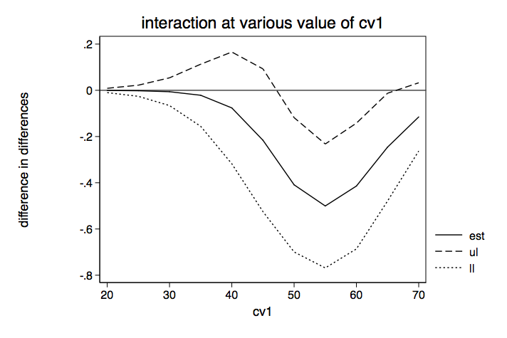
Clearly, the value of the covariate makes a huge difference in whether or not the simple main effects or the interactions are statistically significant when working in the probability metric.
Model 1a: Categorical by categorical interaction?
But wait, what if the model does not contain an interaction term? Consider the following model.
logit y01 i.f i.h cv1 Logistic regression Number of obs = 200 LR chi2(3) = 100.26 Prob > chi2 = 0.0000 Log likelihood = -81.6618 Pseudo R2 = 0.3804 ------------------------------------------------------------------------------ y01 | Coef. Std. Err. z P>|z| [95% Conf. Interval] -------------+---------------------------------------------------------------- 1.f | 1.65172 .4229992 3.90 0.000 .8226566 2.480783 1.h | 1.256555 .4009757 3.13 0.002 .4706575 2.042453 cv1 | .1806214 .0304036 5.94 0.000 .1210314 .2402113 _cons | -10.26943 1.622842 -6.33 0.000 -13.45015 -7.088723 ------------------------------------------------------------------------------
We will manually compute the expected log odds for each of the four cells of the model.
f h cell 0 0 b[_cons] = -10.26943 cell 1 0 b[_cons] + b[1.f] = -10.26943 + 1.65172 = -8.61771 cell 0 1 b[_cons] + b[1.h] = -10.26943 + 1.256555 = -9.012875 cell 1 1 b[_cons] + b[1.f] + b[1.h] = -10.26943 + 1.65172 + 1.256555 = -7.361155
Next we will compute the differences for f=0 and f=1.
difference 1 at f = 0: -10.26943 - -8.6177 = -1.65173 difference 2 at f = 1: -9.012875 - -7.361155 = -1.65172
They are identical to within rounding error, showing that there is no interaction effect in the log odds model.
Next we will compute the expected probabilities for cv1 held at 50 along with the difference in differences.
margins, over(f h) at(cv1=50) post Predictive margins Number of obs = 200 ------------------------------------------------------------------------------ | Delta-method | Margin Std. Err. z P>|z| [95% Conf. Interval] -------------+---------------------------------------------------------------- f#h | 0 0 | .2247204 .0670438 3.35 0.001 .0933171 .3561238 0 1 | .5045471 .0798579 6.32 0.000 .3480285 .6610657 1 0 | .6018917 .0866773 6.94 0.000 .4320073 .7717761 1 1 | .8415636 .0455686 18.47 0.000 .7522509 .9308764 ------------------------------------------------------------------------------ lincom (_b[0.f#1.h]-_b[0.f#0.h])-(_b[1.f#1.h]-_b[1.f#0.h]) ( 1) - 0bn.f#0bn.h + 0bn.f#1.h + 1.f#0bn.h - 1.f#1.h = 0 ------------------------------------------------------------------------------ | Coef. Std. Err. z P>|z| [95% Conf. Interval] -------------+---------------------------------------------------------------- (1) | .0401547 .0364121 1.10 0.270 -.0312117 .111521 ------------------------------------------------------------------------------
The difference in differences is not very large. Let's try in again, this time holding cv1 at 60.
margins, over(f h) at(cv1=60) post Predictive margins Number of obs = 200 ------------------------------------------------------------------------------ | Delta-method | Margin Std. Err. z P>|z| [95% Conf. Interval] -------------+---------------------------------------------------------------- f#h | 0 0 | .6382663 .1046912 6.10 0.000 .4330753 .8434572 0 1 | .8610935 .0455552 18.90 0.000 .7718069 .9503802 1 0 | .9019929 .0470231 19.18 0.000 .8098294 .9941565 1 1 | .9700007 .0146765 66.09 0.000 .9412353 .998766 ------------------------------------------------------------------------------ lincom (_b[0.f#1.h]-_b[0.f#0.h])-(_b[1.f#1.h]-_b[1.f#0.h]) ( 1) - 0bn.f#0bn.h + 0bn.f#1.h + 1.f#0bn.h - 1.f#1.h = 0 ------------------------------------------------------------------------------ | Coef. Std. Err. z P>|z| [95% Conf. Interval] -------------+---------------------------------------------------------------- (1) | .1548195 .0634635 2.44 0.015 .0304334 .2792057 ------------------------------------------------------------------------------
This time the difference in differences is much larger. Let's make a graph similar to the one we did for the model with the interaction included.
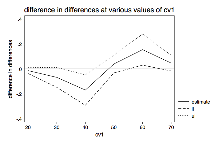
We see that, even without an interaction term in the model, the differences in differences (interactions?) can vary widely from negative to positive depending on the value of the covariate.
This leads us to the "Quote of the Day."
Quote of the day
Departures from additivity imply the presence of interaction types, but additivity does not imply the absence of interaction types.
Greenland & Rothman, 1998
Model 2: Categorical by continuous interaction
Log odds metric — categorical by continuous interaction
The dataset for the categorical by continuous interaction has one binary predictor (f), one continuous predictor (s) and a continuous covariate (cv1). Let's take a look at the logistic regression model.
logit y f##c.s cv1 Logistic regression Number of obs = 200 LR chi2(4) = 114.41 Prob > chi2 = 0.0000 Log likelihood = -74.587842 Pseudo R2 = 0.4340 ------------------------------------------------------------------------------ y | Coef. Std. Err. z P>|z| [95% Conf. Interval] -------------+---------------------------------------------------------------- 1.f | 9.983662 3.05269 3.27 0.001 4.0005 15.96682 s | .1750686 .0470033 3.72 0.000 .0829438 .2671933 | f#c.s | 1 | -.1595233 .0570352 -2.80 0.005 -.2713103 -.0477363 | cv1 | .1877164 .0347888 5.40 0.000 .1195316 .2559013 _cons | -19.00557 3.371064 -5.64 0.000 -25.61273 -12.39841 ------------------------------------------------------------------------------
The interaction term is significant indicating the the slopes for y on s are significantly different for each level of f. We can compute the slopes and intercepts manually as shown below.
slope for f=0: b[s] = .1750686 slope for f=1: b[s] + b[f#c.s] = .1750686 -.1595233 = .0155453 intercept for f=0: _cons = -19.00557 intercept for f=1: _cons + b[1.f]= -19.00557 + 9.983662 = -9.021909
Here are our two logistic regression equations in the log odds metric.
-19.00557 + .1750686*s + 0*cv1 -9.021909 + .0155453*s + 0*cv1
Now we can graph these two regression lines to get an idea of what is going on.
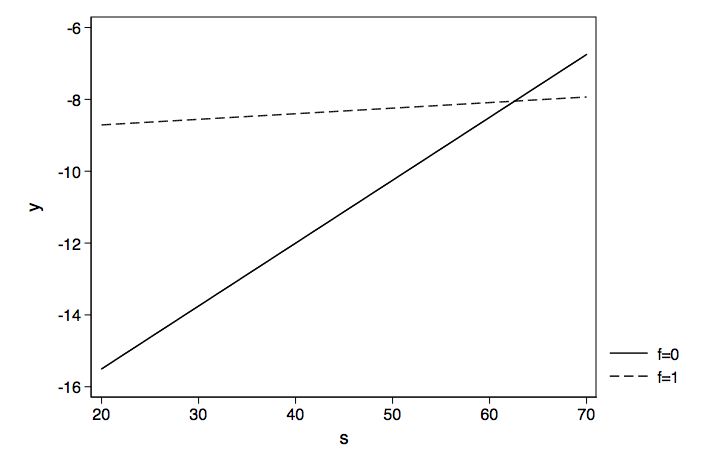
Because the logistic regress model is linear in log odds, the predicted slopes do not change with differing values of the covariate.
Probability metric — categorical by continuous interaction
We'll begin by rerunning the logistic regression model.
logit y f##c.s cv1 Logistic regression Number of obs = 200 LR chi2(4) = 114.41 Prob > chi2 = 0.0000 Log likelihood = -74.587842 Pseudo R2 = 0.4340 ------------------------------------------------------------------------------ y | Coef. Std. Err. z P>|z| [95% Conf. Interval] -------------+---------------------------------------------------------------- 1.f | 9.983662 3.05269 3.27 0.001 4.0005 15.96682 s | .1750686 .0470033 3.72 0.000 .0829438 .2671933 | f#c.s | 1 | -.1595233 .0570352 -2.80 0.005 -.2713103 -.0477363 | cv1 | .1877164 .0347888 5.40 0.000 .1195316 .2559013 _cons | -19.00557 3.371064 -5.64 0.000 -25.61273 -12.39841 ------------------------------------------------------------------------------
If we were so inclined we could compute all of the probabilities of interest using the basic probability formula.
Prob = exp(Xb)/(1+exp(Xb))
Here's an example of computing the probability when f = 0, s = 60, f#s = 0, and cv1 =40.
Xb0 = -19.00557 + 0*9.983662 + 60*.1750686 + 0*-.1595233 + 40*.1877164 = -.992798 exp(Xb0)/(1+exp(Xb0)) = exp(-.992798)/(1+exp(-.992798)) = .27035977
Now we will use f = 1, s = 60, f#s = 60, and cv1 =40.
Xb1 = -19.00557 + 1*9.983662 + 60*.1750686 + 60*-.1595233 + 40*.1877164 = -.580534 exp(Xb1)/(1+exp(Xb1)) = exp(-.580534)/(1+exp(-.580534)) = .35880973
We can also compute the difference in probabilities.
exp(Xb1)/(1+exp(Xb1)) - exp(Xb0)/(1+exp(Xb0)) = exp(-.580534)/(1+exp(-.580534)) - exp(-.992798)/(1+exp(-.992798)) = .08844995
If we use something like Stata's margins command, we can get predicted probabilities along with standard errors and confidence intervals. Here is an example predicting the probability when s = 20 and cv1 = 40.
margins f, at(s=20 cv1=40) Adjusted predictions Number of obs = 200 Model VCE : OIM Expression : Pr(y), predict() ------------------------------------------------------------------------------ | Delta-method | Margin Std. Err. z P>|z| [95% Conf. Interval] -------------+---------------------------------------------------------------- f | 0 | .0003368 .0005779 0.58 0.560 -.0007958 .0014695 1 | .2310582 .1500289 1.54 0.124 -.0629931 .5251095 ------------------------------------------------------------------------------
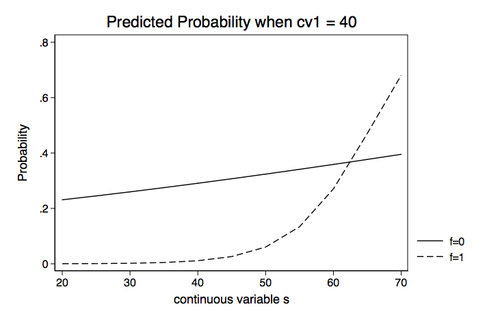
Now can repeat this for various values of s running from 20 to 70, producing the table below.
Table of Predicted Probabilities of f for Various Values of s Holding cv1 at 40 | Delta-method | Margin Std. Err. z P>|z| [95% Conf. Interval] -------------+---------------------------------------------------------------- s f | 20 0 | .0003368 .0005779 0.58 0.560 -.0007958 .0014695 20 1 | .2310582 .1500289 1.54 0.124 -.0629931 .5251095 25 0 | .000808 .0012067 0.67 0.503 -.0015571 .003173 25 1 | .2451555 .1320954 1.86 0.063 -.0137469 .5040578 30 0 | .0019367 .0024706 0.78 0.433 -.0029056 .0067789 30 1 | .2598222 .1136085 2.29 0.022 .0371536 .4824908 35 0 | .0046348 .0049337 0.94 0.348 -.005035 .0143047 35 1 | .2750467 .0959104 2.87 0.004 .0870657 .4630276 40 0 | .0110505 .0095531 1.16 0.247 -.0076733 .0297743 40 1 | .2908127 .081642 3.56 0.000 .1307973 .4508282 45 0 | .0261139 .0178944 1.46 0.144 -.0089585 .0611863 45 1 | .3070997 .0752299 4.08 0.000 .1596518 .4545475 50 0 | .0604557 .0329478 1.83 0.067 -.0041208 .1250322 50 1 | .3238822 .0808248 4.01 0.000 .1654685 .4822959 55 0 | .1337569 .0622149 2.15 0.032 .0118178 .2556959 55 1 | .3411303 .0980782 3.48 0.001 .1489005 .5333601 60 0 | .2703596 .1168105 2.31 0.021 .0414151 .499304 60 1 | .3588096 .1233704 2.91 0.004 .117008 .6006111 65 0 | .4706697 .180248 2.61 0.009 .11739 .8239493 65 1 | .3768809 .1535731 2.45 0.014 .0758831 .6778787 70 0 | .6808947 .1951477 3.49 0.000 .2984123 1.063377 70 1 | .3953013 .1867987 2.12 0.034 .0291827 .7614199 ------------------------------------------------------------------------------
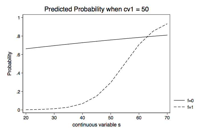
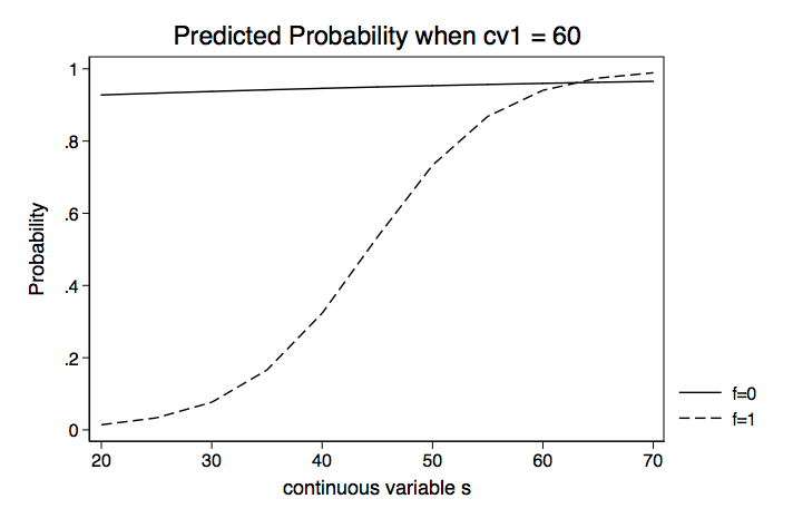
We will repeat this holding cv1 at 50 and then 60. We will then plot the probabilities for each of the three values of cv1.
Instead of looking at separate values for f0 and f1, we could compute the difference in probabilities. Here is an example using margins with the dydx option.
margins, dydx(f) at(s=20 cv1=40) Conditional marginal effects Number of obs = 200 Model VCE : OIM Expression : Pr(y), predict() dy/dx w.r.t. : 1.f at : s = 20 cv1 = 40 ------------------------------------------------------------------------------ | Delta-method | dy/dx Std. Err. z P>|z| [95% Conf. Interval] -------------+---------------------------------------------------------------- 1.f | .2307214 .150045 1.54 0.124 -.0633615 .5248042 ------------------------------------------------------------------------------ Note: dy/dx for factor levels is the discrete change from the base level.
Okay, let's repeat this for different values of s, producing the table below.
Table of Differences in Probability for Various Values of s Holding cv1 at 40 | Delta-method | dy/dx Std. Err. z P>|z| [95% Conf. Interval] -------------+---------------------------------------------------------------- s | 20 | .2307214 .150045 1.54 0.124 -.0633615 .5248042 25 | .2443475 .1321009 1.85 0.064 -.0145655 .5032605 30 | .2578855 .1135271 2.27 0.023 .0353765 .4803946 35 | .2704118 .0954463 2.83 0.005 .0833405 .4574832 40 | .2797622 .0798258 3.50 0.000 .1233066 .4362179 45 | .2809858 .0696338 4.04 0.000 .1445061 .4174655 50 | .2634265 .0682395 3.86 0.000 .1296795 .3971735 55 | .2073734 .0822883 2.52 0.012 .0460913 .3686556 60 | .08845 .1291224 0.69 0.493 -.1646253 .3415252 65 | -.0937888 .2006804 -0.47 0.640 -.4871151 .2995376 70 | -.2855934 .2436296 -1.17 0.241 -.7630986 .1919118 ------------------------------------------------------------------------------ Note: dy/dx for factor levels is the discrete change from the base level.
Next, we need to repeat the process while holding cv1 at 50 and then 60. Then we can plot the differences in probabilities for the three values of cv1 on a single graph.
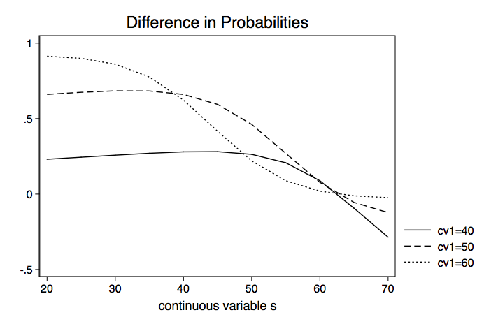
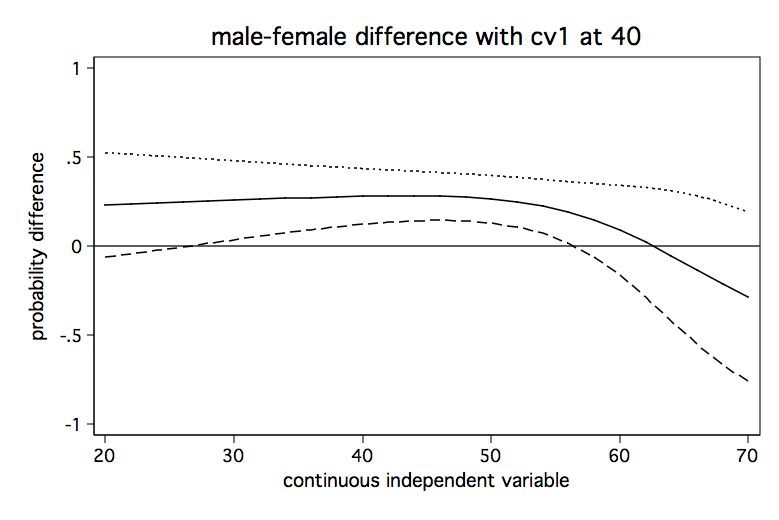
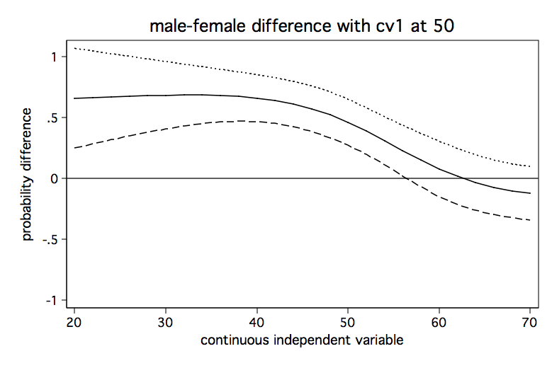
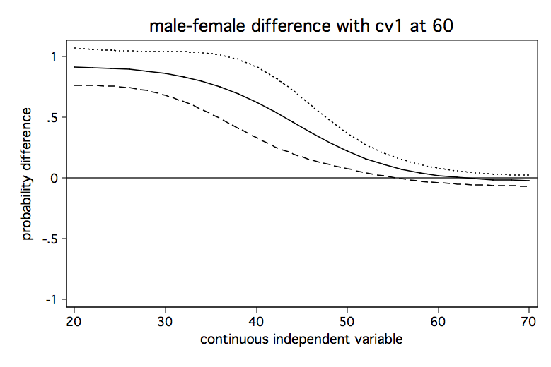
The Stata FAQ page, How can I understand a categorical by continuous interaction in logistic regression? shows an alternative method for graphing these difference in probability lines to include confidence intervals. Here are the graphs from that FAQ page.
Model 3: Continuous by continuous interaction
Log odds metric — continuous by continuous interaction
This time we have a dataset that has two continuous predictors (r & m) and a continuous covariate (cv1).
logit y c.r##c.m cv1, nolog Logistic regression Number of obs = 200 LR chi2(4) = 66.80 Prob > chi2 = 0.0000 Log likelihood = -77.953857 Pseudo R2 = 0.3000 ------------------------------------------------------------------------------ y | Coef. Std. Err. z P>|z| [95% Conf. Interval] -------------+---------------------------------------------------------------- r | .4342063 .1961642 2.21 0.027 .0497316 .8186809 m | .5104617 .2011856 2.54 0.011 .1161452 .9047782 | c.r#c.m | -.0068144 .0033337 -2.04 0.041 -.0133483 -.0002805 | cv1 | .0309685 .0271748 1.14 0.254 -.0222931 .08423 _cons | -34.09122 11.73402 -2.91 0.004 -57.08947 -11.09297 ------------------------------------------------------------------------------
The trick to interpreting continuous by continuous interactions is to fix one predictor at a given value and to vary the other predictor. Once again, since the log odds model is a linear model it really doesn't matter what value the covariate is held at; the slopes do not change. For convenience we will just hold cv1 at zero.
Here is an example manual computation of the slope of r holding m at 30.
slope = b[r] + 30*b[r#m] = .43420626 + 30*(-.00681441) = .22977396
Here is the same computation using Stata.
margins, dydx(r) at(m=30) predict(xb) Average marginal effects Number of obs = 200 Model VCE : OIM Expression : Linear prediction, predict(xb) dy/dx w.r.t. : r at : m = 30 cv1 = 0 ------------------------------------------------------------------------------ | Delta-method | dy/dx Std. Err. z P>|z| [95% Conf. Interval] -------------+---------------------------------------------------------------- r | .2297741 .0982943 2.34 0.019 .0371207 .4224274 ------------------------------------------------------------------------------
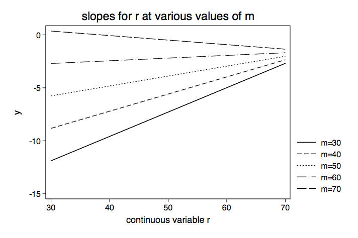
The table below shows the slope for r for various values of m running from 30 to 70. Since this is a linear model we do not have to hold cv1 at any particular value.
Table of Slopes for r for Various Values of m | Delta-method | dy/dx Std. Err. z P>|z| [95% Conf. Interval] -------------+---------------------------------------------------------------- m | 30 | .2297741 .0982943 2.34 0.019 .0371207 .4224274 40 | .16163 .0670895 2.41 0.016 .0301369 .2931231 50 | .0934859 .0395342 2.36 0.018 .0160004 .1709715 60 | .0253419 .0291137 0.87 0.384 -.0317199 .0824037 70 | -.0428022 .0485281 -0.88 0.378 -.1379156 .0523112 ------------------------------------------------------------------------------
We arbitrarily chose to vary m and look at the slope of r but we could have easily reversed the variables. Hopefully, your knowledge of the theory behind the model along with substantive knowledge will suggest which variable to manipulate.
Below is a graph of the slopes from the table above.
This time we are going to move directly to the probability interpretation by-passing the odds ratio metric.
Probability metric — continuous by continuous interaction
We will rerun our model.
logit y c.r##c.m cv1, nolog Logistic regression Number of obs = 200 LR chi2(4) = 66.80 Prob > chi2 = 0.0000 Log likelihood = -77.953857 Pseudo R2 = 0.3000 ------------------------------------------------------------------------------ y | Coef. Std. Err. z P>|z| [95% Conf. Interval] -------------+---------------------------------------------------------------- r | .4342063 .1961642 2.21 0.027 .0497316 .8186809 m | .5104617 .2011856 2.54 0.011 .1161452 .9047782 | c.r#c.m | -.0068144 .0033337 -2.04 0.041 -.0133483 -.0002805 | cv1 | .0309685 .0271748 1.14 0.254 -.0222931 .08423 _cons | -34.09122 11.73402 -2.91 0.004 -57.08947 -11.09297 ------------------------------------------------------------------------------
Next we will calculate the values of the covariate for the mean minus one standard deviation, the mean, and the mean plus one standard deviation.
summarize cv1 Variable | Obs Mean Std. Dev. Min Max -------------+-------------------------------------------------------- cv1 | 200 52.405 10.73579 26 71 mean cv1 - 1sd = 41.669207 mean cv1 = 52.405 mean cv1 + 1sd = 63.140793
Here is an example of a computation for the slope of r in the probability metric for m = 30 hold cv1 at its mean minus 1 sd (41.669207).
margins, dydx(r) at(m=30 cv1=41.669207) Average marginal effects Number of obs = 200 Model VCE : OIM Expression : Pr(y), predict() dy/dx w.r.t. : r at : m = 30 cv1 = 41.66921 ------------------------------------------------------------------------------ | Delta-method | dy/dx Std. Err. z P>|z| [95% Conf. Interval] -------------+---------------------------------------------------------------- r | .0061133 .0065712 0.93 0.352 -.006766 .0189926 ------------------------------------------------------------------------------
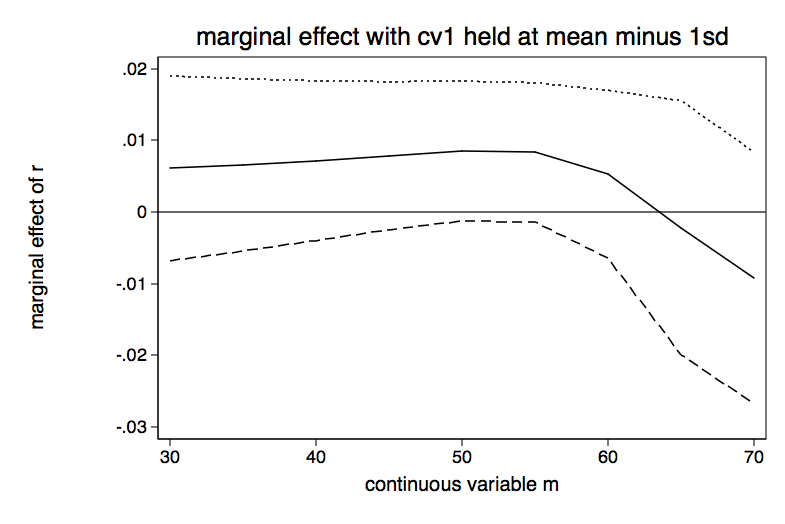
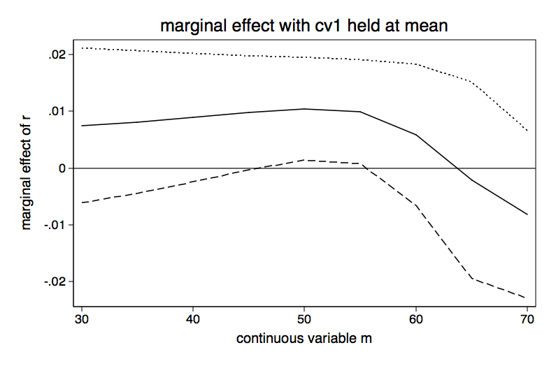
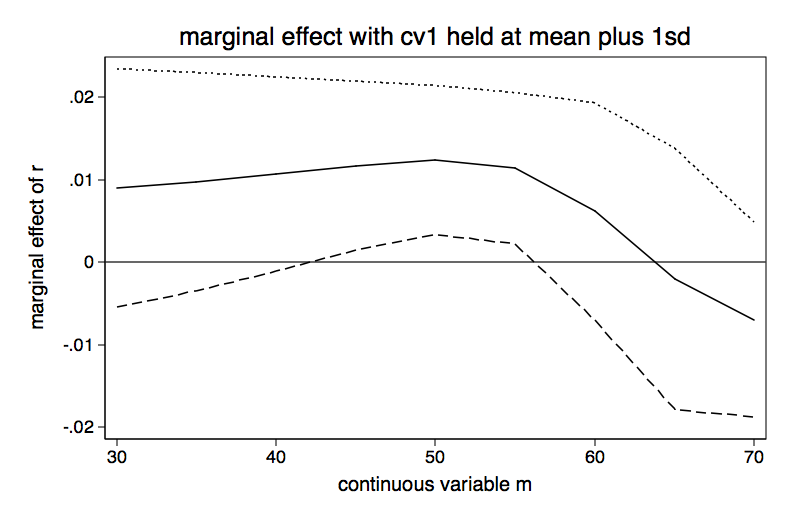
We will now compute the slopes for r for differing values of m for each of the three values of cv1.
Table for Slope of r for Various Values of m holding cv1 at mean minus 1 sd | Delta-method | dy/dx Std. Err. z P>|z| [95% Conf. Interval] -------------+---------------------------------------------------------------- m | 30 | .0061133 .0065712 0.93 0.352 -.006766 .0189926 35 | .006587 .0061377 1.07 0.283 -.0054427 .0186167 40 | .0071815 .0056839 1.26 0.206 -.0039586 .0183217 45 | .0078851 .0052656 1.50 0.134 -.0024354 .0182055 50 | .0085235 .004981 1.71 0.087 -.0012391 .0182861 55 | .0083341 .0049614 1.68 0.093 -.0013901 .0180583 60 | .0052692 .0059747 0.88 0.378 -.0064411 .0169795 65 | -.002175 .0090427 -0.24 0.810 -.0198984 .0155484 70 | -.0091967 .0089699 -1.03 0.305 -.0267774 .0083839 ------------------------------------------------------------------------------ Table for Slope of r for Various Values of m holding cv1 at the mean -------------+---------------------------------------------------------------- 30 | .0074917 .0069416 1.08 0.280 -.0061135 .0210969 35 | .0081075 .0063953 1.27 0.205 -.004427 .0206421 40 | .0088605 .0057648 1.54 0.124 -.0024384 .0201593 45 | .009721 .0051157 1.90 0.057 -.0003056 .0197476 50 | .0104242 .0046175 2.26 0.024 .0013739 .0194744 55 | .00992 .0046688 2.12 0.034 .0007692 .0190708 60 | .0058498 .006339 0.92 0.356 -.0065745 .0182741 65 | -.0021432 .0088189 -0.24 0.808 -.019428 .0151416 70 | -.0081533 .0075364 -1.08 0.279 -.0229243 .0066177 ------------------------------------------------------------------------------ Table for Slope of r for Various Values of m holding cv1 at mean plus 1 sd -------------+---------------------------------------------------------------- m | 30 | .0090189 .0073769 1.22 0.221 -.0054396 .0234774 35 | .0097902 .0067546 1.45 0.147 -.0034485 .0230289 40 | .0107094 .0060155 1.78 0.075 -.0010807 .0224994 45 | .0117184 .0052384 2.24 0.025 .0014513 .0219854 50 | .0124196 .0046088 2.69 0.007 .0033864 .0214527 55 | .0114027 .004686 2.43 0.015 .0022182 .0205871 60 | .006181 .0067253 0.92 0.358 -.0070003 .0193622 65 | -.0020011 .0080879 -0.25 0.805 -.0178531 .0138509 70 | -.0069432 .0060361 -1.15 0.250 -.0187739 .0048874
We will graph each of the three tables above.
The bottom line
- Just because the interaction term is significant in the log odds model, it doesn't mean that the probability difference in differences will be significant for values of the covariate of interest.
- Paradoxically, even if the interaction term is not significant in the log odds model, the probability difference in differences may be significant for some values of the covariate.
- In the probability metric the values of all the variables in the model matter.
References
Ai, C.R. and Norton E.C. 2003. Interaction terms in logit and probit models. Economics Letters 80(1): 123-129.
Greenland, S. and Rothman, K.J. 1998. Modern Epidemiology, 2nd Ed. Philadelphia: Lippincott Williams and Wilkins.
Mitchell, M.N. and Chen X. 2005. Visualizing main effects and interactions for binary logit model. Stata Journal 5(1): 64-82.
Norton, E.C., Wang, H., and Ai, C. 2004 Computing interaction effects and standard errors in logit and probit models. Stata Journal 4(2): 154-167.
Comma separated data files
Categorical by categorical: https://stats.idre.ucla.edu/wp-content/uploads/2016/02/concon2.csv
Categorical by continuous: https://stats.idre.ucla.edu/wp-content/uploads/2016/02/logitcatcon.csv
Continuous by continuous: https://stats.idre.ucla.edu/wp-content/uploads/2016/02/logitconcon.csv
Source: https://stats.oarc.ucla.edu/stata/seminars/deciphering-interactions-in-logistic-regression/
0 Response to "Interpreting Odds Ratios for Continuous Variables in Logistic Regression"
Post a Comment